Processing Data From Scratch
… with Bowman (2018) data.
In this tutorial, we will go through an entire processing of a subset of the data going into the Bowman et al. (2018) Nature paper. The point here is not to reproduce the exact results (note: there is an effort to do this that you can follow). It is rather to show the various steps involved from a users perspective, and justify some of those choices.
The point is also not to provide a full mathematical description and justification of all the procedures. That will be done elsewhere (pending…). The point is to give you enough of a description that you have a high level idea of what’s going on, and then also to show you how to use the code to achieve it. We will also focus a little on the expected workflow – running a processing step, visualising the results, and iterating.
High-level overview
Before getting into any actual calculations, let’s go over what the purpose of edges-analysis is, and what it essentially does.
The purpose of the analysis part of edges-analysis is to take existing raw spectrum data, measured in the field, and process it down to a set of averaged spectra, which can subsequently be fit with some cosmological and foreground model(s) using `edges-estimate <https://github.com/edges-collab/edges-estimate>`__.
There are three main aspects to this processing:
Calibration – applying a linear transformation to each recorded spectrum to convert it from a set of recorded powers to a physical temperature.
Filtering – the process of identifying and flagging bad data (whether due to unstable instrument, environmental conditions, or RFI).
Averaging/Integrating – the process of combining different recorded spectra in a consistent way to improve the signal-to-noise.
One thing to note is that the entire process is almost linear. That is, if we were to apply a different calibration, then do all the filtering and averaging, then invert the initial calibration and apply a different one, it would be almost the same as having just initially applied the different calibration. It is only almost the same because the identification of bad data in the filtering step can rely on the calibrated temperature to some degree.
Though there are three aspects, these are not standalone “steps” in their own right, as if we could just do “calibrate” then “filter” then “average”. For one, each aspect has multiple ways of performing it, eg. in “calibration” we need to do the lab-based gain calibration, but also need to correct for losses and the beam chromaticity. Likewise, in “filtering” we can filter on total recorded power, RFI, humidity, etc.
Furthermore, while the calibration routines are all typically applied first, it is generally useful to alternate between filtering and averaging: filter some, average a little more to expose more bad data, filter some more, … etc. Nevertheless, a lot of the kinds of filtering are most useful before any averaging is done (i.e. on the raw calibrated spectra) – eg. filtering out high humidity, or filtering on the position of the sun/moon.
So, given all that, here’s the general process as a list of steps:
Calibrate, including:
Lab-based gain calibration (requiring calibration solutions to be determined elsewhere)
Loss corrections from the balun, ground and antenna.
Beam chromaticity correction
Initial filtering, including:
Filtering entire spectra based on auxiliary data (sun/moon/humidity/temperature)
Filtering entire spectra based on a prior of total measured power
RFI filtering
Filtering entire spectra based on the RMS of low-order fits
Average each night’s spectra into small, regular bins of LST/GHA.
At the same time, collect all the nights together into one array, shape
(nights, gha, frequency).Then do another round of RFI filtering on the averaged data!
Average over the nights
Leaving an array of shape
(gha, frequency).Filter RFI again!
Successively average within larger GHA bins
Wise to do this a little at a time, doing more RFI flagging with each integration.
Final product still
(gha, frequency), but with larger GHA bins (as desired).
Code Overview
So, we have the general steps involved. How does one use edges-analysis to achieve this? Before digging into details and actually performing this analysis, let’s have a quick high-level look at the code.
‘Step’ Objects
Each of the basic steps above are encoded as classes/objects within edges-analysis. These objects all have a very similar interface, and have a few cool features:
They store all the parameters that go into doing the processing, so that you can go back and reproduce it any time.
They have a
write()method that writes down all the data into a HDF5 file with a nice structure that is also able to be easily read by the same object.They know about one another – you can
promote()one set of data to the next step.If you write each step to file, the steps further down the chain know who their parents are, and can go and dynamically look up data associated with the parents.
Thus, if you write each step to file, in principle the final step has all the information about the whole process available, including every parameter used to define it.
There is a Command-Line Interface (CLI) that intelligently writes each step to file for you, using a self-consistent file layout.
To be clear, the available steps (in order) are:
There is an extra step here: the ModelData. As it turns out, all the averaging we do relies on having some fiducial model of each spectrum, so as to make an unbiased average in the presence of non-uniform weights. So, we fit a model to each un-averaged spectrum at the beginning, and carry through those models and their residuals to the following steps.
Note also that every step has the opportunity to perform RFI filtering (not just FilteredData).
In addition to these basic step objects, some of the steps require external input, like beam and sky models. There are classes for these in their respective modules, and we will refer to them as they come up.
General Workflow
In general, the workflow for the processing is as follows:
Write a YAML settings file defining the inputs to a particular step
Run the CLI for that step, inputting files from the previous step (or raw spectra if its the first step), and using the YAML settings.
Open up the written file in a notebook/python script with the
read_stepfunction, and make some plots that show the state of the data. Use this to decide whether to rerun the previous step again with different parameters (or even higher-up steps), and to inform what settings you might want to put on the next step.Repeat from (1) for each step, until you get to the
BinnedData.
Note that some of the steps can be run more than once, in particular the FilteredData and BinnedData. That is you can run multiple filters progressively, and bin progressively. Furthermore, the FilteredData step can be skipped entirely (though it is not advisable).
Compute Intensity
It helps your workflow to understand where the most processing time occurs. Though it is somewhat dependent on your parameter choices, typically the most intensive step is the FilteredData, due to the RFI extraction on all individual spectra. If doing RFI extraction on the the CombinedData, it is typically the next slowest, followed by CalibratedData. The other steps are generally quite fast, and can be rerun quickly to explore different parameters.
Let’s Process Some Data…!
Now that we have an overview, let’s dive in and do some data processing, using the workflow of switching between the CLI and the notebook. Fortunately, you can run things on the CLI within a notebook!
The data we will be using is a subset of the data that went into the Nature paper, so that we proceed relatively quickly. Note that this tutorial will assume that we are running on the enterprise server on which the raw data is stored. As long as you have the data on your machine, and your paths set correctly, it will work wherever you run it.
All the settings files used here are stored in the config directory in the Github repo (go ahead and click that link), so you can access them as well.
First, let’s import some of the functions that we’ll need. Importantly, we’ll need the read_step function, which is able to read any file defined as one of the analysis steps:
[140]:
from edges_analysis import read_step

%matplotlib inline
import matplotlib.pyplot as plt
import numpy as np
from copy import deepcopy
%load_ext autoreload
%autoreload 2
The autoreload extension is already loaded. To reload it, use:
  %reload_ext autoreload
Setting Up
Before we dive into the actual processing, let’s review our overall setup. Since many files are required to do a calibration – the raw input spectra, the \(S_{11}\) measurements of the antenna, auxiliary measurements of humidity etc., beam files, etc., – edges-analysis provides a central location to configure where those different things might be found:
[2]:
from edges_analysis import cfg
[3]:
cfg
[3]:
{'paths': {'antenna': '/home/smurray/edges/Steven/edges-cache/antenna-models',
  'beams': '/home/smurray/edges/Steven/edges-cache/beam-models',
  'field_products': '/home/smurray/edges/Steven/edges-cache/level-cache',
  'lab_products': '/home/smurray/edges/Steven/edges-cache/calibration-cache',
  'raw_field_data': '/data5/edges/data/2014_February_Boolardy',
  'raw_lab_data': '/data4/edges/data/CalibrationObservations',
  'sky_models': '/home/smurray/data4/edges-sky-models/'}}
Changing any of these paths will change the global behaviour of the package. You can also write this config to disk to make that change permanent!
[4]:
cfg.write()
Importantly, throughout you will see that some input paths are prefixed by :. This is a context-aware identifier that points to the default location of a given kind of input, according to the configuration. Eg. passing a beam model path in any function as :/my_beam.feko will be interpreted as cfg['paths']['beams'] / my_beam.feko.
Calibration
Let’s first look at our settings:
[5]:
!cat config/calibrate.yml
band: low
f_low: 50
f_high: 100
calfile: /data4/smurray/cal_file_Rcv01_2015_09.h5
s11_path: /data5/edges/data/S11_antenna/low_band/20160830_a/s11
balun_correction: true
antenna_correction: false
ground_correction: ':'
beam_file: /home/nmahesh/edges-beams/low/beam_factors/feko_Haslam408_ref70.00_22f61e7c4b66d33e811dc6825b04001a.h5
The first question is: how do you know what parameters are available, and what they mean? The answer is to look at the input parameters to the promote method of the relevant class – in this case, CalibratedData.promote. Anything defined there (except the prev_step input itself) can be included in the YAML settings.
Now, what are these settings?
We are using low band data (specifically, the low-band2 antenna), and we would like to restrict our attention to the 50-100 MHz band (the intrinsic data goes down to 40 MHz and up to 200 MHz, but the quality of the calibration is extremely poor outside this region).
The calfile is a bit more tricky – clearly it points to an external file. This file is a representation of an edges_cal.Calibration object, which you must produce yourself prior to running edges-analysis (or get it from someone else). In particular, the calibration observation we are using comes from a lab run in September 2015 – the same calibration used in the Nature Paper results.
The s11_path points to a directory of \(S_{11}\) measurements taken in the field. In this directory are four files, each of which is required to produce the corrected \(S_{11}\) function. In general, the directory may have many more files – so long as those files follow a reasonable filename convention with the dates they were obtained, the code will find the measurements closest to each measured spectra, and use those to calibrate.
The balun and antenna corrections are analytic corrections that are built-in to the code. The original NP results did not use an antenna correction, and neither do we here. The ground correction however does require an externally-produced model of the ground plane loss. There is no code in edges-analysis to create this file, however, a reasonable default for the low-band is included in the code itself, so passing “:” just finds this default file.
Finally, the beam_file points to a file representing a beams.InterpolatedBeamFactor object. This also must be created before running the calibration, however code for doing so is included in edges-analysis. We do not show how to do it here, but point you to THIS TUTORIAL (coming…).
Finally, we must decide on our input files. We will use days 2016-290 – 2016-310 (20 days of data). We run the command as following. Note that -i gives the input files (and we use the “:” notation to refer to the default location of spectra on enterprise). We give -i multiple times, and all the files it finds will be processed. Futhermore, each of them has a * in it – a glob wildcard.
We also give -l, which sets the label for these settings, and also is the output directory into which the results will be saved. Finally, we give -j to specify the number of processes to use in parallel.
[10]:
!edges-analysis process calibrate config/calibrate.yml \
  -i :2016/2016_29* -i :2016/2016_30* \
  -l nature-paper-subset \
  -j 20
╔══════════════════════════════════════════════════════════════════════════════╗
║                           edges-analysis calibrate                           ║
╚══════════════════════════════════════════════════════════════════════════════╝
────────────────────────────────── Setting Up ──────────────────────────────────

                                    Settings
┏━━━━━━━━━━━━━━━━━━━━┳━━━━━━━━━━━━━━━━━━━━━━━━━━━━━━━━━━━━━━━━━━━━━━━━━━━━━━━━━┓
┃ band               ┃ low                                                     ┃
│ f_low              │ 50                                                      │
│ f_high             │ 100                                                     │
│ calfile            │ /data4/smurray/cal_file_Rcv01_2015_09.h5                │
│ s11_path           │ /data5/edges/data/S11_antenna/low_band/20160830_a/s11   │
│ balun_correction   │ True                                                    │
│ antenna_correction │ False                                                   │
│ ground_correction  │ :                                                       │
│ beam_file          │ /home/nmahesh/edges-beams/low/beam_factors/feko_Haslam… │
└────────────────────┴─────────────────────────────────────────────────────────┘

Input Files:
   /data5/edges/data/2014_February_Boolardy/mro/low/2016/2016_291_00.acq
   /data5/edges/data/2014_February_Boolardy/mro/low/2016/2016_298_00.acq
   /data5/edges/data/2014_February_Boolardy/mro/low/2016/2016_294_00.acq
   /data5/edges/data/2014_February_Boolardy/mro/low/2016/2016_296_00.acq
   /data5/edges/data/2014_February_Boolardy/mro/low/2016/2016_299_00.acq
   /data5/edges/data/2014_February_Boolardy/mro/low/2016/2016_293_00.acq
   /data5/edges/data/2014_February_Boolardy/mro/low/2016/2016_290_00.acq
   /data5/edges/data/2014_February_Boolardy/mro/low/2016/2016_297_00.acq
   /data5/edges/data/2014_February_Boolardy/mro/low/2016/2016_295_00.acq
   /data5/edges/data/2014_February_Boolardy/mro/low/2016/2016_292_00.acq
   /data5/edges/data/2014_February_Boolardy/mro/low/2016/2016_304_00.acq
   /data5/edges/data/2014_February_Boolardy/mro/low/2016/2016_302_14.acq
   /data5/edges/data/2014_February_Boolardy/mro/low/2016/2016_303_00.acq
   /data5/edges/data/2014_February_Boolardy/mro/low/2016/2016_305_00.acq

Output Directory:
/home/smurray/edges/Steven/edges-cache/level-cache/nature-paper-subset

───────────────────────────── Beginning Processing ─────────────────────────────
  0%|                                                 | 0/14 [00:00<?, ?files/s]INFO     Time for reading: 0.00 sec.
INFO     Converting time strings to datetimes...
INFO     ...  finished in 0.02 sec.
INFO     Getting ancillary weather data...
INFO     Setting up arrays...
INFO     .... took 0.0004076957702636719 sec.
INFO     Took 0.001993417739868164 sec to interpolate auxiliary data.
INFO     Took 0.27565932273864746 sec to get lst/gha
INFO     Time for reading: 0.00 sec.
INFO     Converting time strings to datetimes...
INFO     ...  finished in 0.02 sec.
INFO     Getting ancillary weather data...
INFO     Setting up arrays...
INFO     .... took 0.0005230903625488281 sec.
INFO     Took 0.0022695064544677734 sec to interpolate auxiliary data.
INFO     Took 0.15206098556518555 sec to get lst/gha
INFO     Took 3.2985928058624268 sec to get sun/moon coords.
INFO     ... finished in 6.37 sec.
INFO     Calibrating data ...
INFO     Took 3.530212163925171 sec to get sun/moon coords.
INFO     ... finished in 3.84 sec.
INFO     Calibrating data ...
/data4/smurray/Projects/radio/EOR/Edges/edges-analysis/src/edges_analysis/analysis/levels.py:1552: RankWarning: Polyfit may be poorly conditioned
  switch_state_repeat_num=switch_state_repeat_num,
/data4/smurray/Projects/radio/EOR/Edges/edges-analysis/src/edges_analysis/analysis/levels.py:1552: RankWarning: Polyfit may be poorly conditioned
  switch_state_repeat_num=switch_state_repeat_num,
/data4/smurray/Projects/radio/EOR/Edges/edges-analysis/src/edges_analysis/analysis/levels.py:1552: RankWarning: Polyfit may be poorly conditioned
  switch_state_repeat_num=switch_state_repeat_num,
/data4/smurray/Projects/radio/EOR/Edges/edges-analysis/src/edges_analysis/analysis/levels.py:1552: RankWarning: Polyfit may be poorly conditioned
  switch_state_repeat_num=switch_state_repeat_num,
INFO     ... finished in 2.55 sec.
INFO     ... finished in 5.85 sec.
 14%|█████▊                                   | 2/14 [00:31<04:17, 21.50s/files]INFO     Time for reading: 0.00 sec.
INFO     Converting time strings to datetimes...
INFO     ...  finished in 0.04 sec.
INFO     Getting ancillary weather data...
INFO     Setting up arrays...
INFO     .... took 0.0016689300537109375 sec.
INFO     Took 0.0071790218353271484 sec to interpolate auxiliary data.
INFO     Took 0.41275572776794434 sec to get lst/gha
INFO     Time for reading: 0.00 sec.
INFO     Converting time strings to datetimes...
INFO     ...  finished in 0.05 sec.
INFO     Getting ancillary weather data...
INFO     Setting up arrays...
INFO     .... took 0.0011680126190185547 sec.
INFO     Took 0.005935192108154297 sec to interpolate auxiliary data.
INFO     Took 0.3269069194793701 sec to get lst/gha
INFO     Took 7.115918159484863 sec to get sun/moon coords.
INFO     ... finished in 7.71 sec.
INFO     Calibrating data ...
INFO     Time for reading: 0.00 sec.
INFO     Converting time strings to datetimes...
INFO     ...  finished in 0.05 sec.
INFO     Getting ancillary weather data...
/data4/smurray/Projects/radio/EOR/Edges/edges-analysis/src/edges_analysis/analysis/levels.py:1552: RankWarning: Polyfit may be poorly conditioned
  switch_state_repeat_num=switch_state_repeat_num,
/data4/smurray/Projects/radio/EOR/Edges/edges-analysis/src/edges_analysis/analysis/levels.py:1552: RankWarning: Polyfit may be poorly conditioned
  switch_state_repeat_num=switch_state_repeat_num,
INFO     Setting up arrays...
INFO     .... took 0.002516031265258789 sec.
INFO     Took 0.01175689697265625 sec to interpolate auxiliary data.
INFO     Time for reading: 0.00 sec.
INFO     Converting time strings to datetimes...
INFO     ...  finished in 0.05 sec.
INFO     Getting ancillary weather data...
INFO     Setting up arrays...
INFO     .... took 0.0012021064758300781 sec.
INFO     Took 0.005623340606689453 sec to interpolate auxiliary data.
INFO     Took 0.5263016223907471 sec to get lst/gha
INFO     Time for reading: 0.00 sec.
INFO     Converting time strings to datetimes...
INFO     ...  finished in 0.05 sec.
INFO     Getting ancillary weather data...
INFO     Took 0.33168506622314453 sec to get lst/gha
INFO     Setting up arrays...
INFO     .... took 0.0021936893463134766 sec.
INFO     Took 0.009093761444091797 sec to interpolate auxiliary data.
INFO     Time for reading: 0.00 sec.
INFO     Converting time strings to datetimes...
INFO     ...  finished in 0.05 sec.
INFO     Getting ancillary weather data...
INFO     Setting up arrays...
INFO     .... took 0.002326488494873047 sec.
INFO     Took 0.007919549942016602 sec to interpolate auxiliary data.
INFO     Took 0.34461283683776855 sec to get lst/gha
INFO     Time for reading: 0.00 sec.
INFO     Converting time strings to datetimes...
INFO     ...  finished in 0.05 sec.
INFO     Getting ancillary weather data...
INFO     Setting up arrays...
INFO     .... took 0.0010981559753417969 sec.
INFO     Took 0.004992246627807617 sec to interpolate auxiliary data.
INFO     Time for reading: 0.00 sec.
INFO     Converting time strings to datetimes...
INFO     ...  finished in 0.05 sec.
INFO     Getting ancillary weather data...
INFO     Time for reading: 0.00 sec.
INFO     Converting time strings to datetimes...
INFO     ...  finished in 0.04 sec.
INFO     Getting ancillary weather data...
INFO     Took 0.4826779365539551 sec to get lst/gha
INFO     Setting up arrays...
INFO     .... took 0.0011532306671142578 sec.
INFO     Took 0.005100727081298828 sec to interpolate auxiliary data.
INFO     Setting up arrays...
INFO     .... took 0.0011589527130126953 sec.
INFO     Took 0.004923582077026367 sec to interpolate auxiliary data.
INFO     Time for reading: 0.00 sec.
INFO     Converting time strings to datetimes...
INFO     ...  finished in 0.05 sec.
INFO     Getting ancillary weather data...
INFO     Took 0.4586927890777588 sec to get lst/gha
INFO     Setting up arrays...
INFO     .... took 0.002145528793334961 sec.
INFO     Took 0.008849620819091797 sec to interpolate auxiliary data.
INFO     Took 0.32550764083862305 sec to get lst/gha
INFO     Took 0.3024122714996338 sec to get lst/gha
INFO     Took 0.3883779048919678 sec to get lst/gha
INFO     Time for reading: 0.00 sec.
INFO     Converting time strings to datetimes...
INFO     ...  finished in 0.07 sec.
INFO     Getting ancillary weather data...
INFO     Setting up arrays...
INFO     .... took 0.0019714832305908203 sec.
INFO     Took 0.008300065994262695 sec to interpolate auxiliary data.
INFO     Time for reading: 0.00 sec.
INFO     Converting time strings to datetimes...
INFO     ...  finished in 0.07 sec.
INFO     Getting ancillary weather data...
INFO     Setting up arrays...
INFO     .... took 0.002028942108154297 sec.
INFO     Took 0.008279085159301758 sec to interpolate auxiliary data.
INFO     Took 0.5257954597473145 sec to get lst/gha
INFO     ... finished in 4.00 sec.
INFO     Took 0.48622679710388184 sec to get lst/gha
 21%|████████▊                                | 3/14 [01:02<04:29, 24.49s/files]INFO     Took 9.269782543182373 sec to get sun/moon coords.
INFO     ... finished in 9.79 sec.
INFO     Calibrating data ...
/data4/smurray/Projects/radio/EOR/Edges/edges-analysis/src/edges_analysis/analysis/levels.py:1552: RankWarning: Polyfit may be poorly conditioned
  switch_state_repeat_num=switch_state_repeat_num,
/data4/smurray/Projects/radio/EOR/Edges/edges-analysis/src/edges_analysis/analysis/levels.py:1552: RankWarning: Polyfit may be poorly conditioned
  switch_state_repeat_num=switch_state_repeat_num,
INFO     Took 7.862194538116455 sec to get sun/moon coords.
INFO     ... finished in 8.39 sec.
INFO     Calibrating data ...
/data4/smurray/Projects/radio/EOR/Edges/edges-analysis/src/edges_analysis/analysis/levels.py:1552: RankWarning: Polyfit may be poorly conditioned
  switch_state_repeat_num=switch_state_repeat_num,
/data4/smurray/Projects/radio/EOR/Edges/edges-analysis/src/edges_analysis/analysis/levels.py:1552: RankWarning: Polyfit may be poorly conditioned
  switch_state_repeat_num=switch_state_repeat_num,
INFO     Took 7.180325746536255 sec to get sun/moon coords.
INFO     ... finished in 7.64 sec.
INFO     Calibrating data ...
/data4/smurray/Projects/radio/EOR/Edges/edges-analysis/src/edges_analysis/analysis/levels.py:1552: RankWarning: Polyfit may be poorly conditioned
  switch_state_repeat_num=switch_state_repeat_num,
/data4/smurray/Projects/radio/EOR/Edges/edges-analysis/src/edges_analysis/analysis/levels.py:1552: RankWarning: Polyfit may be poorly conditioned
  switch_state_repeat_num=switch_state_repeat_num,
INFO     Took 8.789221286773682 sec to get sun/moon coords.
INFO     ... finished in 9.30 sec.
INFO     Calibrating data ...
/data4/smurray/Projects/radio/EOR/Edges/edges-analysis/src/edges_analysis/analysis/levels.py:1552: RankWarning: Polyfit may be poorly conditioned
  switch_state_repeat_num=switch_state_repeat_num,
/data4/smurray/Projects/radio/EOR/Edges/edges-analysis/src/edges_analysis/analysis/levels.py:1552: RankWarning: Polyfit may be poorly conditioned
  switch_state_repeat_num=switch_state_repeat_num,
INFO     Took 9.446529150009155 sec to get sun/moon coords.
INFO     ... finished in 10.22 sec.
INFO     Calibrating data ...
/data4/smurray/Projects/radio/EOR/Edges/edges-analysis/src/edges_analysis/analysis/levels.py:1552: RankWarning: Polyfit may be poorly conditioned
  switch_state_repeat_num=switch_state_repeat_num,
/data4/smurray/Projects/radio/EOR/Edges/edges-analysis/src/edges_analysis/analysis/levels.py:1552: RankWarning: Polyfit may be poorly conditioned
  switch_state_repeat_num=switch_state_repeat_num,
INFO     Took 8.51799488067627 sec to get sun/moon coords.
INFO     ... finished in 9.18 sec.
INFO     Calibrating data ...
INFO     Took 8.327298641204834 sec to get sun/moon coords.
INFO     ... finished in 8.82 sec.
INFO     Calibrating data ...
/data4/smurray/Projects/radio/EOR/Edges/edges-analysis/src/edges_analysis/analysis/levels.py:1552: RankWarning: Polyfit may be poorly conditioned
  switch_state_repeat_num=switch_state_repeat_num,
/data4/smurray/Projects/radio/EOR/Edges/edges-analysis/src/edges_analysis/analysis/levels.py:1552: RankWarning: Polyfit may be poorly conditioned
  switch_state_repeat_num=switch_state_repeat_num,
INFO     Took 8.01357102394104 sec to get sun/moon coords.
INFO     ... finished in 8.58 sec.
INFO     Calibrating data ...
/data4/smurray/Projects/radio/EOR/Edges/edges-analysis/src/edges_analysis/analysis/levels.py:1552: RankWarning: Polyfit may be poorly conditioned
  switch_state_repeat_num=switch_state_repeat_num,
/data4/smurray/Projects/radio/EOR/Edges/edges-analysis/src/edges_analysis/analysis/levels.py:1552: RankWarning: Polyfit may be poorly conditioned
  switch_state_repeat_num=switch_state_repeat_num,
/data4/smurray/Projects/radio/EOR/Edges/edges-analysis/src/edges_analysis/analysis/levels.py:1552: RankWarning: Polyfit may be poorly conditioned
  switch_state_repeat_num=switch_state_repeat_num,
/data4/smurray/Projects/radio/EOR/Edges/edges-analysis/src/edges_analysis/analysis/levels.py:1552: RankWarning: Polyfit may be poorly conditioned
  switch_state_repeat_num=switch_state_repeat_num,
INFO     Took 8.769074201583862 sec to get sun/moon coords.
INFO     ... finished in 9.40 sec.
INFO     Calibrating data ...
/data4/smurray/Projects/radio/EOR/Edges/edges-analysis/src/edges_analysis/analysis/levels.py:1552: RankWarning: Polyfit may be poorly conditioned
  switch_state_repeat_num=switch_state_repeat_num,
/data4/smurray/Projects/radio/EOR/Edges/edges-analysis/src/edges_analysis/analysis/levels.py:1552: RankWarning: Polyfit may be poorly conditioned
  switch_state_repeat_num=switch_state_repeat_num,
INFO     Took 7.868443012237549 sec to get sun/moon coords.
INFO     ... finished in 8.57 sec.
INFO     Calibrating data ...
/data4/smurray/Projects/radio/EOR/Edges/edges-analysis/src/edges_analysis/analysis/levels.py:1552: RankWarning: Polyfit may be poorly conditioned
  switch_state_repeat_num=switch_state_repeat_num,
/data4/smurray/Projects/radio/EOR/Edges/edges-analysis/src/edges_analysis/analysis/levels.py:1552: RankWarning: Polyfit may be poorly conditioned
  switch_state_repeat_num=switch_state_repeat_num,
INFO     ... finished in 3.44 sec.
INFO     ... finished in 3.33 sec.
INFO     ... finished in 3.45 sec.
INFO     ... finished in 3.39 sec.
INFO     Took 9.332679271697998 sec to get sun/moon coords.
INFO     ... finished in 10.12 sec.
INFO     Calibrating data ...
INFO     ... finished in 3.58 sec.
/data4/smurray/Projects/radio/EOR/Edges/edges-analysis/src/edges_analysis/analysis/levels.py:1552: RankWarning: Polyfit may be poorly conditioned
  switch_state_repeat_num=switch_state_repeat_num,
/data4/smurray/Projects/radio/EOR/Edges/edges-analysis/src/edges_analysis/analysis/levels.py:1552: RankWarning: Polyfit may be poorly conditioned
  switch_state_repeat_num=switch_state_repeat_num,
INFO     ... finished in 3.50 sec.
INFO     ... finished in 3.55 sec.
INFO     ... finished in 3.99 sec.
INFO     ... finished in 4.02 sec.
INFO     ... finished in 5.38 sec.
INFO     ... finished in 3.76 sec.
100%|████████████████████████████████████████| 14/14 [01:20<00:00,  5.72s/files]
─────────────────────────────── Done Processing ────────────────────────────────

All files written to:
/home/smurray/edges/Steven/edges-cache/level-cache/nature-paper-subset
Calibrating these 14 files took only about a minute and a half. Note the informative output we received, especially the last line, which tells us where the output is stored. Let’s read one of those files:
[6]:
cal_step = read_step("/home/smurray/edges/Steven/edges-cache/level-cache/nature-paper-subset/2016-290-00.h5")
While you can look at the online API docs to see everything we have access to in this object, you can also use interactive help by pressing tab.
A few important things you have access to are the .spectrum:
[7]:
cal_step.spectrum.shape
[7]:
(2270, 8192)
the ancillary data:
[8]:
print(list(cal_step.ancillary.keys()))
['adcmax', 'adcmin', 'ambient_hum', 'ambient_temp', 'frontend_temp', 'gha', 'lna_temp', 'lst', 'moon_az', 'moon_el', 'power_percent', 'rack_temp', 'receiver_temp', 'seconds', 'sun_az', 'sun_el', 'temp_set', 'times']
the frequencies:
[9]:
cal_step.raw_frequencies.shape
[9]:
(8192,)
and the metadata:
[10]:
print(cal_step.meta.keys())
dict_keys(['antenna_correction', 'antenna_s11_n_terms', 'balun_correction', 'band', 'beam_file', 'calfile', 'calobs_path', 'configuration', 'cterms', 'day', 'edges_analysis_version', 'edges_io_version', 'f_high', 'f_low', 'freq_max', 'freq_min', 'freq_res', 'ground_correction', 'hour', 'ignore_s11_files', 'leave_progress', 'message', 'n_file_lines', 'nblk', 'nfreq', 'object_name', 'out_file', 'parent_files', 'progress', 'resolution', 's11_file_pattern', 's11_files', 's11_path', 'switch_state_dir', 'switch_state_repeat_num', 'temperature', 'thermlog_file', 'weather_file', 'write_time', 'wterms', 'xrfi_pipe', 'year'])
Perhaps most important are various plotting functions that allow you to inspect the data:
[11]:
cal_step.plot_waterfall(vmax=10000);
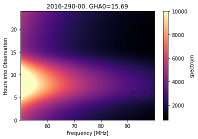
Immediately here we notice some bad RFI at high frequencies around the 5th hour of observation.
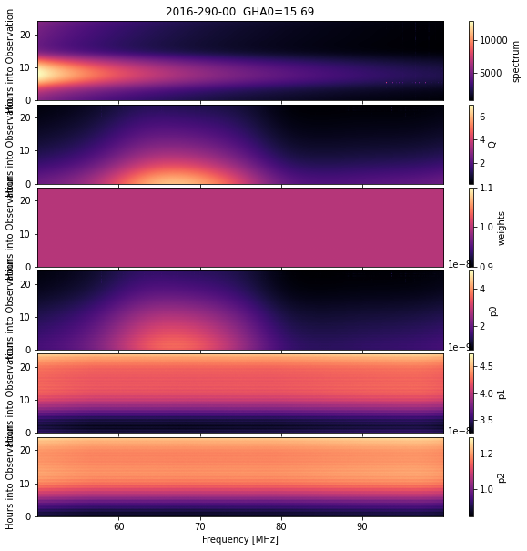
Since the data comes from the combination of three measured switch powers, we can plot all of those:
[18]:
cal_step.plot_waterfalls();
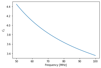
Finally, we can access the underlying calibration object, eg:
[26]:
plt.plot(cal_step.raw_frequencies, cal_step.calibration.C1(cal_step.raw_frequencies))
plt.ylabel("$C_1$")
plt.xlabel("Frequency [MHz]");
Filtering
Let’s have a look at our filtering configuration:
[27]:
!cat config/filter1.yml
# Filter on auxiliary information
sun_el_max: -10
moon_el_max: 90
ambient_humidity_max: 40
min_receiver_temp: 0
max_receiver_temp: 100

do_total_power_filter: true
n_poly_tp_filter: 3
n_sigma_tp_filter: 3.0
bands_tp_filter: null # whole band

negative_power_filter: true

# How to filter out RFI
xrfi_pipe:
  xrfi_model:
    model_type: linlog
    beta: -2.5
    max_iter: 15
    increase_order: true
    threshold: 6
    decrement_threshold: 1
    min_threshold: 4
    min_terms: 4
    max_terms: 7
    n_signal: 3
    n_resid: 3
    watershed: 4
    init_flags: [90., 100.0]

  xrfi_watershed:
    tol: 0.7


n_threads: 32
The first category of filters are the auxiliary information – these are fairly self-explanatory. Notably, here we ensure the sun is well below the horizon, but do not filter on the moon’s position. We also require reasonably dry conditions.
The second category is the total_power_filter. This fits a function to the average power over the whole band as a function of time, and finds significant outliers. The parameters control the number of parameters in the fit to the function, and the significance of the outliers that are cut.
The third – and most complex – category is the RFI. Here, we pass a series of methods to use (xrfi_model then xrfi_watershed). These are names of functions in edges_cal.xrfi. Then we pass parameters to each. Here, we are relying primarily on xrfi_model, which will fit a simple model to each spectrum, and treat the absolute residuals as a measure of the standard deviation, with which it will start to flag outliers. It is a bit more complicated than this; it does this
iteratively, finding flags, then a better model, then more flags, etc. Each iteration, the number of parameters in the fit may change, or the threshold. The watershed argument means that we flag channels around the flagged channels, in order to be conservative. The init_flags set a region in frequency that are flagged for the initial fit, so that really bad RFI doesn’t adversely affect the initial conditions of the iteration.
So, let’s run this. Notice that the CLI call is very similar to the one for calibration. However, we pass a different settings file, and give the input as a colon-prefixed pointer to the label we gave to the calibration step. Since this is a directory, it will read all the .h5 files in that directory. Our label here is aux-tp-xrfi-model, which essentially captures the filters we’re using.
[28]:
!edges-analysis process filter config/filter1.yml \
  -i :nature-paper-subset \
  -l aux-tp-xrfi-model \
  -j 14
╔══════════════════════════════════════════════════════════════════════════════╗
║                            edges-analysis filter                             ║
╚══════════════════════════════════════════════════════════════════════════════╝
────────────────────────────────── Setting Up ──────────────────────────────────

                                    Settings
┏━━━━━━━━━━━━━━━━━━━━━━━┳━━━━━━━━━━━━━━━━━━━━━━━━━━━━━━━━━━━━━━━━━━━━━━━━━━━━━━┓
┃ sun_el_max            ┃ -10                                                  ┃
│ moon_el_max           │ 90                                                   │
│ ambient_humidity_max  │ 40                                                   │
│ min_receiver_temp     │ 0                                                    │
│ max_receiver_temp     │ 100                                                  │
│ do_total_power_filter │ True                                                 │
│ n_poly_tp_filter      │ 3                                                    │
│ n_sigma_tp_filter     │ 3.0                                                  │
│ bands_tp_filter       │ None                                                 │
│ negative_power_filter │ True                                                 │
│ xrfi_pipe             │ {'xrfi_model': {'model_type': 'linlog', 'beta':      │
│                       │ -2.5, 'max_iter': 15, 'increase_order': True,        │
│                       │ 'threshold': 6, 'decrement_threshold': 1,            │
│                       │ 'min_threshold': 4, 'min_terms': 4, 'max_terms': 7,  │
│                       │ 'n_signal': 3, 'n_resid': 3, 'watershed': 4,         │
│                       │ 'init_flags': [90.0, 100.0]}, 'xrfi_watershed':      │
│                       │ {'tol': 0.7}}                                        │
│ n_threads             │ 32                                                   │
└───────────────────────┴──────────────────────────────────────────────────────┘

Input Files:
   /home/smurray/edges/Steven/edges-cache/level-cache/nature-paper-subset/2016-2
98-00.h5
   /home/smurray/edges/Steven/edges-cache/level-cache/nature-paper-subset/2016-3
02-14.h5
   /home/smurray/edges/Steven/edges-cache/level-cache/nature-paper-subset/2016-2
93-00.h5
   /home/smurray/edges/Steven/edges-cache/level-cache/nature-paper-subset/2016-2
91-00.h5
   /home/smurray/edges/Steven/edges-cache/level-cache/nature-paper-subset/2016-2
92-00.h5
   /home/smurray/edges/Steven/edges-cache/level-cache/nature-paper-subset/2016-2
90-00.h5
   /home/smurray/edges/Steven/edges-cache/level-cache/nature-paper-subset/2016-2
94-00.h5
   /home/smurray/edges/Steven/edges-cache/level-cache/nature-paper-subset/2016-2
97-00.h5
   /home/smurray/edges/Steven/edges-cache/level-cache/nature-paper-subset/2016-3
03-00.h5
   /home/smurray/edges/Steven/edges-cache/level-cache/nature-paper-subset/2016-3
04-00.h5
   /home/smurray/edges/Steven/edges-cache/level-cache/nature-paper-subset/2016-2
96-00.h5
   /home/smurray/edges/Steven/edges-cache/level-cache/nature-paper-subset/2016-3
05-00.h5
   /home/smurray/edges/Steven/edges-cache/level-cache/nature-paper-subset/2016-2
99-00.h5
   /home/smurray/edges/Steven/edges-cache/level-cache/nature-paper-subset/2016-2
95-00.h5

Output Directory: /home/smurray/edges/Steven/edges-cache/level-cache/nature-pape
r-subset/aux-tp-xrfi-model

───────────────────────────── Beginning Processing ─────────────────────────────
INFO     Running aux filter.
INFO     Running aux filter.
INFO     Running aux filter.
  0%|                                                 | 0/14 [00:00<?, ?files/s]INFO     Running aux filter.
INFO     Running aux filter.
INFO     Running aux filter.
INFO     Running aux filter.
INFO     Running aux filter.
INFO     Running aux filter.
INFO     Running aux filter.
INFO     Running aux filter.
INFO     Running aux filter.
INFO     Running aux filter.
INFO     Running aux filter.
INFO     '2016-290-00.h5': 0.00 → 58.99% <+58.99%> flagged after 'aux' filter
INFO     Running negative_power filter.
INFO     '2016-290-00.h5': 58.99 → 58.99% <+0.00%> flagged after
         'negative_power' filter
INFO     Running rfi filter.
INFO     '2016-302-14.h5': 0.00 → 36.12% <+36.12%> flagged after 'aux' filter
INFO     Running negative_power filter.
WARNING  2016-299-00.h5 was fully flagged during aux filter
INFO     Running negative_power filter.
INFO     Running rfi filter.
INFO     Running total_power filter.
INFO     '2016-302-14.h5': 36.12 → 36.12% <+0.00%> flagged after
         'negative_power' filter
INFO     Running rfi filter.
WARNING  2016-304-00.h5 was fully flagged during aux filter
INFO     Running negative_power filter.
WARNING  2016-294-00.h5 was fully flagged during aux filter
INFO     Running negative_power filter.
WARNING  2016-303-00.h5 was fully flagged during aux filter
INFO     Running negative_power filter.
INFO     Running rfi filter.
INFO     Running rfi filter.
INFO     Running rfi filter.
INFO     Running total_power filter.
INFO     Running total_power filter.
INFO     Running total_power filter.
INFO     '2016-291-00.h5': 0.00 → 59.11% <+59.11%> flagged after 'aux' filter
INFO     Running negative_power filter.
INFO     '2016-293-00.h5': 0.00 → 59.35% <+59.35%> flagged after 'aux' filter
INFO     Running negative_power filter.
INFO     '2016-297-00.h5': 0.00 → 59.81% <+59.81%> flagged after 'aux' filter
INFO     Running negative_power filter.
INFO     '2016-292-00.h5': 0.00 → 59.29% <+59.29%> flagged after 'aux' filter
INFO     Running negative_power filter.
INFO     '2016-298-00.h5': 0.00 → 59.97% <+59.97%> flagged after 'aux' filter
INFO     Running negative_power filter.
INFO     '2016-305-00.h5': 0.00 → 54.70% <+54.70%> flagged after 'aux' filter
INFO     Running negative_power filter.
INFO     '2016-296-00.h5': 0.00 → 59.68% <+59.68%> flagged after 'aux' filter
INFO     Running negative_power filter.
INFO     '2016-295-00.h5': 0.00 → 59.59% <+59.59%> flagged after 'aux' filter
INFO     Running negative_power filter.
  7%|██▉                                      | 1/14 [00:03<00:39,  3.03s/files]INFO     '2016-305-00.h5': 54.70 → 54.70% <+0.00%> flagged after
         'negative_power' filter
INFO     Running rfi filter.
INFO     '2016-291-00.h5': 59.11 → 59.11% <+0.00%> flagged after
         'negative_power' filter
INFO     Running rfi filter.
INFO     '2016-292-00.h5': 59.29 → 59.29% <+0.00%> flagged after
         'negative_power' filter
INFO     Running rfi filter.
INFO     '2016-296-00.h5': 59.68 → 59.68% <+0.00%> flagged after
         'negative_power' filter
INFO     Running rfi filter.
INFO     '2016-297-00.h5': 59.81 → 59.81% <+0.00%> flagged after
         'negative_power' filter
INFO     Running rfi filter.
INFO     '2016-295-00.h5': 59.59 → 59.59% <+0.00%> flagged after
         'negative_power' filter
INFO     Running rfi filter.
INFO     '2016-293-00.h5': 59.35 → 59.35% <+0.00%> flagged after
         'negative_power' filter
INFO     Running rfi filter.
 21%|████████▊                                | 3/14 [00:05<00:23,  2.10s/files]INFO     '2016-298-00.h5': 59.97 → 59.97% <+0.00%> flagged after
         'negative_power' filter
INFO     Running rfi filter.
bool
INFO     2016-291-00: After xrfi_model, nflags=11013457/18571264 (59.3%)
bool
INFO     2016-291-00: After xrfi_watershed, nflags=11033942/18571264 (59.4%)
INFO     '2016-291-00.h5': 59.11 → 59.41% <+0.31%> flagged after 'rfi' filter
INFO     Running total_power filter.
INFO     '2016-291-00.h5': 59.41 → 59.92% <+0.51%> flagged after 'total_power'
         filter
 36%|██████████████▋                          | 5/14 [02:08<02:59, 19.92s/files]bool
INFO     2016-296-00: After xrfi_model, nflags=11151783/18571264 (60.0%)
bool
INFO     2016-296-00: After xrfi_watershed, nflags=11193048/18571264 (60.3%)
INFO     '2016-296-00.h5': 59.68 → 60.27% <+0.59%> flagged after 'rfi' filter
INFO     Running total_power filter.
INFO     '2016-296-00.h5': 60.27 → 60.82% <+0.55%> flagged after 'total_power'
         filter
 43%|█████████████████▌                       | 6/14 [02:33<02:51, 21.39s/files]bool
INFO     2016-302-14: After xrfi_model, nflags=2586174/6963200 (37.1%)
bool
INFO     2016-302-14: After xrfi_watershed, nflags=2589714/6963200 (37.2%)
INFO     '2016-302-14.h5': 36.12 → 37.19% <+1.07%> flagged after 'rfi' filter
INFO     Running total_power filter.
INFO     '2016-302-14.h5': 37.19 → 38.23% <+1.04%> flagged after 'total_power'
         filter
 50%|████████████████████▌                    | 7/14 [03:25<03:33, 30.46s/files]bool
INFO     2016-295-00: After xrfi_model, nflags=11099359/18571264 (59.8%)
bool
INFO     2016-295-00: After xrfi_watershed, nflags=11119112/18571264 (59.9%)
INFO     '2016-295-00.h5': 59.59 → 59.87% <+0.28%> flagged after 'rfi' filter
INFO     Running total_power filter.
INFO     '2016-295-00.h5': 59.87 → 60.25% <+0.38%> flagged after 'total_power'
         filter
 57%|███████████████████████▍                 | 8/14 [03:59<03:08, 31.44s/files]bool
INFO     2016-305-00: After xrfi_model, nflags=8752740/15933440 (54.9%)
bool
INFO     2016-305-00: After xrfi_watershed, nflags=8772111/15933440 (55.1%)
INFO     '2016-305-00.h5': 54.70 → 55.05% <+0.35%> flagged after 'rfi' filter
INFO     Running total_power filter.
INFO     '2016-305-00.h5': 55.05 → 55.51% <+0.45%> flagged after 'total_power'
         filter
 64%|██████████████████████████▎              | 9/14 [04:21<02:23, 28.69s/files]bool
INFO     2016-293-00: After xrfi_model, nflags=11081495/18579456 (59.6%)
bool
INFO     2016-290-00: After xrfi_model, nflags=11038835/18595840 (59.4%)
bool
INFO     2016-293-00: After xrfi_watershed, nflags=11122985/18579456 (59.9%)
bool
INFO     '2016-293-00.h5': 59.35 → 59.87% <+0.52%> flagged after 'rfi' filter
INFO     Running total_power filter.
INFO     2016-290-00: After xrfi_watershed, nflags=11073340/18595840 (59.5%)
INFO     '2016-290-00.h5': 58.99 → 59.55% <+0.56%> flagged after 'rfi' filter
INFO     Running total_power filter.
INFO     '2016-290-00.h5': 59.55 → 60.02% <+0.47%> flagged after 'total_power'
         filter
INFO     '2016-293-00.h5': 59.87 → 60.33% <+0.47%> flagged after 'total_power'
         filter
bool
INFO     2016-297-00: After xrfi_model, nflags=11180042/18571264 (60.2%)
 79%|███████████████████████████████▍        | 11/14 [04:42<00:55, 18.59s/files]bool
INFO     2016-297-00: After xrfi_watershed, nflags=11216240/18571264 (60.4%)
INFO     '2016-297-00.h5': 59.81 → 60.40% <+0.58%> flagged after 'rfi' filter
INFO     Running total_power filter.
INFO     '2016-297-00.h5': 60.40 → 60.78% <+0.39%> flagged after 'total_power'
         filter
bool
INFO     2016-292-00: After xrfi_model, nflags=11118056/18571264 (59.9%)
bool
INFO     2016-292-00: After xrfi_watershed, nflags=11153537/18571264 (60.1%)
INFO     '2016-292-00.h5': 59.29 → 60.06% <+0.77%> flagged after 'rfi' filter
INFO     Running total_power filter.
 86%|██████████████████████████████████▎     | 12/14 [04:47<00:28, 14.31s/files]INFO     '2016-292-00.h5': 60.06 → 60.44% <+0.38%> flagged after 'total_power'
         filter
 93%|█████████████████████████████████████▏  | 13/14 [04:49<00:10, 10.64s/files]bool
INFO     2016-298-00: After xrfi_model, nflags=11212717/18563072 (60.4%)
bool
INFO     2016-298-00: After xrfi_watershed, nflags=11234521/18563072 (60.5%)
INFO     '2016-298-00.h5': 59.97 → 60.52% <+0.55%> flagged after 'rfi' filter
INFO     Running total_power filter.
INFO     '2016-298-00.h5': 60.52 → 60.99% <+0.47%> flagged after 'total_power'
         filter
100%|████████████████████████████████████████| 14/14 [04:51<00:00, 20.85s/files]
─────────────────────────────── Done Processing ────────────────────────────────

Output Files:
        /home/smurray/edges/Steven/edges-cache/level-cache/nature-paper-subset/a
ux-tp-xrfi-model/2016-298-00.h5
        /home/smurray/edges/Steven/edges-cache/level-cache/nature-paper-subset/a
ux-tp-xrfi-model/2016-302-14.h5
        /home/smurray/edges/Steven/edges-cache/level-cache/nature-paper-subset/a
ux-tp-xrfi-model/2016-293-00.h5
        /home/smurray/edges/Steven/edges-cache/level-cache/nature-paper-subset/a
ux-tp-xrfi-model/2016-291-00.h5
        /home/smurray/edges/Steven/edges-cache/level-cache/nature-paper-subset/a
ux-tp-xrfi-model/2016-292-00.h5
        /home/smurray/edges/Steven/edges-cache/level-cache/nature-paper-subset/a
ux-tp-xrfi-model/2016-290-00.h5
        /home/smurray/edges/Steven/edges-cache/level-cache/nature-paper-subset/a
ux-tp-xrfi-model/2016-294-00.h5
        /home/smurray/edges/Steven/edges-cache/level-cache/nature-paper-subset/a
ux-tp-xrfi-model/2016-297-00.h5
        /home/smurray/edges/Steven/edges-cache/level-cache/nature-paper-subset/a
ux-tp-xrfi-model/2016-303-00.h5
        /home/smurray/edges/Steven/edges-cache/level-cache/nature-paper-subset/a
ux-tp-xrfi-model/2016-304-00.h5
        /home/smurray/edges/Steven/edges-cache/level-cache/nature-paper-subset/a
ux-tp-xrfi-model/2016-296-00.h5
        /home/smurray/edges/Steven/edges-cache/level-cache/nature-paper-subset/a
ux-tp-xrfi-model/2016-305-00.h5
        /home/smurray/edges/Steven/edges-cache/level-cache/nature-paper-subset/a
ux-tp-xrfi-model/2016-299-00.h5
        /home/smurray/edges/Steven/edges-cache/level-cache/nature-paper-subset/a
ux-tp-xrfi-model/2016-295-00.h5
Notice that this step took significantly longer (and can take longer still if different xrfi models are used).
Let’s read in one of the files produced:
[29]:
filtered_data = read_step("/home/smurray/edges/Steven/edges-cache/level-cache/nature-paper-subset/aux-tp-xrfi-model/2016-290-00.h5")
Many of the same plotting methods are available here:
[32]:
filtered_data.plot_waterfall();

Notice that a lot of the observation is now flagged (white). We can check which filter gave rise to these flags:
[35]:
fig, ax = plt.subplots(1, 3, sharey=True, figsize=(15, 7))

filtered_data.plot_waterfall(flagged='aux', ax=ax[0])
filtered_data.plot_waterfall(flagged='rfi', ax=ax[1])
filtered_data.plot_waterfall(flagged='tp', ax=ax[2]);
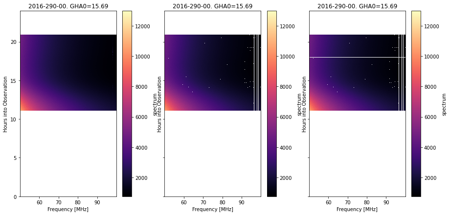
Notice that the auxiliary filter cuts out clean sections of the observation, the RFI filter picks out many spot-like flags, plus some consistent lines in frequency, while the total power filter finds whole bad integrations within the main body of the measurement.
If we had not explicitly read in the calibration file, we could still access that information here:
[36]:
filtered_data.calibration_step
[36]:
CalibratedData(filename=PosixPath('/home/smurray/edges/Steven/edges-cache/level-cache/nature-paper-subset/2016-290-00.h5'), group_path='', require_no_extra=False)
It’s kind of hard to say whether we really got all the bad data in this step. Let’s proceed to the next before we make a judgment.
Modeling
This step is important – we model each individual spectrum with a given smooth model that will help us to do averaging more appropriately in later steps. Having a model also helps us to look more closely at the data, as we can subtract out the model and look at residuals.
[37]:
!cat config/model.yml
model_nterms: 5
model_basis: linlog
model_resolution: 0
The input parameters are very simple here. The point to make is that the kind of model you fit is flexible – it can be anything defined in edges_cal.modelling. Typically, we’ve found that a LinLog model with about 5 terms does pretty well. Finally, the resolution sets the frequency resolution to which the spectra will be binned before fitting the models. Ostensibly, it might be faster to make the resolution larger. However, we typically find that performing the binning is just as
intensive as fitting the model, so there’s really no gain in setting it above zero.
[38]:
!edges-analysis process model config/model.yml \
  -i :nature-paper-subset/aux-tp-xrfi-model \
  -l linlog5-res0 \
  -j 14
╔══════════════════════════════════════════════════════════════════════════════╗
║                             edges-analysis model                             ║
╚══════════════════════════════════════════════════════════════════════════════╝
────────────────────────────────── Setting Up ──────────────────────────────────

          Settings
┏━━━━━━━━━━━━━━━━━━┳━━━━━━━━┓
┃ model_nterms     ┃ 5      ┃
│ model_basis      │ linlog │
│ model_resolution │ 0      │
└──────────────────┴────────┘

Input Files:
   /home/smurray/edges/Steven/edges-cache/level-cache/nature-paper-subset/aux-tp
-xrfi-model/2016-298-00.h5
   /home/smurray/edges/Steven/edges-cache/level-cache/nature-paper-subset/aux-tp
-xrfi-model/2016-302-14.h5
   /home/smurray/edges/Steven/edges-cache/level-cache/nature-paper-subset/aux-tp
-xrfi-model/2016-293-00.h5
   /home/smurray/edges/Steven/edges-cache/level-cache/nature-paper-subset/aux-tp
-xrfi-model/2016-291-00.h5
   /home/smurray/edges/Steven/edges-cache/level-cache/nature-paper-subset/aux-tp
-xrfi-model/2016-292-00.h5
   /home/smurray/edges/Steven/edges-cache/level-cache/nature-paper-subset/aux-tp
-xrfi-model/2016-290-00.h5
   /home/smurray/edges/Steven/edges-cache/level-cache/nature-paper-subset/aux-tp
-xrfi-model/2016-294-00.h5
   /home/smurray/edges/Steven/edges-cache/level-cache/nature-paper-subset/aux-tp
-xrfi-model/2016-297-00.h5
   /home/smurray/edges/Steven/edges-cache/level-cache/nature-paper-subset/aux-tp
-xrfi-model/2016-303-00.h5
   /home/smurray/edges/Steven/edges-cache/level-cache/nature-paper-subset/aux-tp
-xrfi-model/2016-304-00.h5
   /home/smurray/edges/Steven/edges-cache/level-cache/nature-paper-subset/aux-tp
-xrfi-model/2016-296-00.h5
   /home/smurray/edges/Steven/edges-cache/level-cache/nature-paper-subset/aux-tp
-xrfi-model/2016-305-00.h5
   /home/smurray/edges/Steven/edges-cache/level-cache/nature-paper-subset/aux-tp
-xrfi-model/2016-299-00.h5
   /home/smurray/edges/Steven/edges-cache/level-cache/nature-paper-subset/aux-tp
-xrfi-model/2016-295-00.h5

Output Directory: /home/smurray/edges/Steven/edges-cache/level-cache/nature-pape
r-subset/aux-tp-xrfi-model/linlog5-res0

───────────────────────────── Beginning Processing ─────────────────────────────
  0%|                                                 | 0/14 [00:00<?, ?files/s]INFO     Determining 5-term 'linlog' models for each integration...
INFO     Determining 5-term 'linlog' models for each integration...
INFO     Determining 5-term 'linlog' models for each integration...
INFO     Determining 5-term 'linlog' models for each integration...
INFO     Determining 5-term 'linlog' models for each integration...
INFO     Determining 5-term 'linlog' models for each integration...
INFO     Determining 5-term 'linlog' models for each integration...
INFO     Determining 5-term 'linlog' models for each integration...
INFO     Determining 5-term 'linlog' models for each integration...
INFO     Determining 5-term 'linlog' models for each integration...
INFO     Determining 5-term 'linlog' models for each integration...
WARNING
INFO     Determining 5-term 'linlog' models for each integration...
INFO     Determining 5-term 'linlog' models for each integration...
WARNING
INFO     Determining 5-term 'linlog' models for each integration...
WARNING
WARNING
100%|████████████████████████████████████████| 14/14 [00:11<00:00,  1.22files/s]
─────────────────────────────── Done Processing ────────────────────────────────

Output Files:
        /home/smurray/edges/Steven/edges-cache/level-cache/nature-paper-subset/a
ux-tp-xrfi-model/linlog5-res0/2016-298-00.h5
        /home/smurray/edges/Steven/edges-cache/level-cache/nature-paper-subset/a
ux-tp-xrfi-model/linlog5-res0/2016-302-14.h5
        /home/smurray/edges/Steven/edges-cache/level-cache/nature-paper-subset/a
ux-tp-xrfi-model/linlog5-res0/2016-293-00.h5
        /home/smurray/edges/Steven/edges-cache/level-cache/nature-paper-subset/a
ux-tp-xrfi-model/linlog5-res0/2016-291-00.h5
        /home/smurray/edges/Steven/edges-cache/level-cache/nature-paper-subset/a
ux-tp-xrfi-model/linlog5-res0/2016-292-00.h5
        /home/smurray/edges/Steven/edges-cache/level-cache/nature-paper-subset/a
ux-tp-xrfi-model/linlog5-res0/2016-290-00.h5
        /home/smurray/edges/Steven/edges-cache/level-cache/nature-paper-subset/a
ux-tp-xrfi-model/linlog5-res0/2016-294-00.h5
        /home/smurray/edges/Steven/edges-cache/level-cache/nature-paper-subset/a
ux-tp-xrfi-model/linlog5-res0/2016-297-00.h5
        /home/smurray/edges/Steven/edges-cache/level-cache/nature-paper-subset/a
ux-tp-xrfi-model/linlog5-res0/2016-303-00.h5
        /home/smurray/edges/Steven/edges-cache/level-cache/nature-paper-subset/a
ux-tp-xrfi-model/linlog5-res0/2016-304-00.h5
        /home/smurray/edges/Steven/edges-cache/level-cache/nature-paper-subset/a
ux-tp-xrfi-model/linlog5-res0/2016-296-00.h5
        /home/smurray/edges/Steven/edges-cache/level-cache/nature-paper-subset/a
ux-tp-xrfi-model/linlog5-res0/2016-305-00.h5
        /home/smurray/edges/Steven/edges-cache/level-cache/nature-paper-subset/a
ux-tp-xrfi-model/linlog5-res0/2016-299-00.h5
        /home/smurray/edges/Steven/edges-cache/level-cache/nature-paper-subset/a
ux-tp-xrfi-model/linlog5-res0/2016-295-00.h5
As we see – this only took about 11 seconds! Let’s read it in:
[39]:
model_data = read_step("/home/smurray/edges/Steven/edges-cache/level-cache/nature-paper-subset/aux-tp-xrfi-model/linlog5-res0/2016-290-00.h5")
After modelling, we have access to another quantity: the residuals. In fact, only the residuals and model parameters are saved in the data file, not the spectrum. However, the spectrum attribute is still available (it just lazily evaluates the spectrum given the model and residuals).
Let’s make our waterfall again, this time using the residuals:
[47]:
plt.figure(figsize=(15,10))
model_data.plot_waterfall(quantity='resids', ax=plt.gca(), flagged=True);
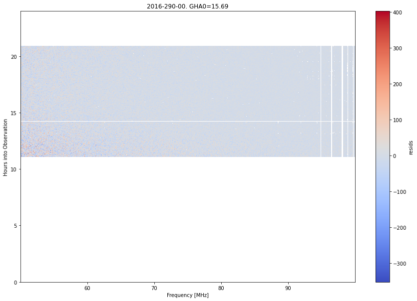
This gives us a bit of a closer view of potentially bad data, and it appears that the data is fairly clean – at these noise levels (still at ~100 K!). Most likely, we must average down a bit further before we can truly understand if we’re getting it all.
GHA Gridding / Combining
Now, we want to combine all the files we have made (one for each day) into a single file with a regular grid of GHA. We want the GHA bin size to be small, so we can still identify small regions of bad data and flag them before they infect everything. Here’s our settings:
[48]:
!cat config/combine.yml
# How to combine the files into a standard grid.
gha_bin_size: 0.05

xrfi_on_resids: false
xrfi_pipe:
  xrfi_model:
    model_type: linlog
    beta: -2.55
    max_iter: 15
    increase_order: true
    threshold: 4.5
    decrement_threshold: 1
    min_threshold: 3.5
    min_terms: 5
    max_terms: 7
    n_signal: 4
    n_resid: 3
    watershed: 4

  xrfi_watershed:
    tol: 0.7
Note here that we really just have to choose our GHA bin size – we set it at 3 minutes. Furthermore, we again provide an RFI filtering scheme, which in fact we keep roughly the same as in the filtering step. The idea here is that lower-level RFI missed in the initial filtering may be caught more easily since we’ve now averaged together about ~6 spectra into each GHA bin. Note that we also set xrfi_on_resids to False. The idea here is that the RFI filtering can happen on the residuals,
or the spectrum. Since we are trying to fit a LinLog model, we want to use the spectra.
Let’s run our now-familiar command-line invocation. The addition here is the -o option, which specifies a name for the single output file. Up til now, each file was uniquely identified by its date, but when combining files, the obvious name would be the concatenation of all the dates, which is impractical. Furthermore, using a hash for a filename would be unique, but they’re so darn hard to remember. So, we ask for a unique label.
Note that we could pass in a subset of the days from the previous step, by again using the glob notation. However, let’s use all the days:
[51]:
!edges-analysis process combine config/combine.yml \
  -i :nature-paper-subset/aux-tp-xrfi-model/linlog5-res0 \
  -l 3min-bins-xrfi-model \
  -j 14 \
  -o all-files
╔══════════════════════════════════════════════════════════════════════════════╗
║                            edges-analysis combine                            ║
╚══════════════════════════════════════════════════════════════════════════════╝
────────────────────────────────── Setting Up ──────────────────────────────────

                                    Settings
┏━━━━━━━━━━━━━━━━┳━━━━━━━━━━━━━━━━━━━━━━━━━━━━━━━━━━━━━━━━━━━━━━━━━━━━━━━━━━━━━┓
┃ gha_bin_size   ┃ 0.05                                                        ┃
│ xrfi_on_resids │ False                                                       │
│ xrfi_pipe      │ {'xrfi_model': {'model_type': 'linlog', 'beta': -2.55,      │
│                │ 'max_iter': 15, 'increase_order': True, 'threshold': 4.5,   │
│                │ 'decrement_threshold': 1, 'min_threshold': 3.5,             │
│                │ 'min_terms': 5, 'max_terms': 7, 'n_signal': 4, 'n_resid':   │
│                │ 3, 'watershed': 4}, 'xrfi_watershed': {'tol': 0.7}}         │
└────────────────┴─────────────────────────────────────────────────────────────┘

Input Files:
   /home/smurray/edges/Steven/edges-cache/level-cache/nature-paper-subset/aux-tp
-xrfi-model/linlog5-res0/2016-298-00.h5
   /home/smurray/edges/Steven/edges-cache/level-cache/nature-paper-subset/aux-tp
-xrfi-model/linlog5-res0/2016-302-14.h5
   /home/smurray/edges/Steven/edges-cache/level-cache/nature-paper-subset/aux-tp
-xrfi-model/linlog5-res0/2016-293-00.h5
   /home/smurray/edges/Steven/edges-cache/level-cache/nature-paper-subset/aux-tp
-xrfi-model/linlog5-res0/2016-291-00.h5
   /home/smurray/edges/Steven/edges-cache/level-cache/nature-paper-subset/aux-tp
-xrfi-model/linlog5-res0/2016-292-00.h5
   /home/smurray/edges/Steven/edges-cache/level-cache/nature-paper-subset/aux-tp
-xrfi-model/linlog5-res0/2016-290-00.h5
   /home/smurray/edges/Steven/edges-cache/level-cache/nature-paper-subset/aux-tp
-xrfi-model/linlog5-res0/2016-297-00.h5
   /home/smurray/edges/Steven/edges-cache/level-cache/nature-paper-subset/aux-tp
-xrfi-model/linlog5-res0/2016-296-00.h5
   /home/smurray/edges/Steven/edges-cache/level-cache/nature-paper-subset/aux-tp
-xrfi-model/linlog5-res0/2016-305-00.h5
   /home/smurray/edges/Steven/edges-cache/level-cache/nature-paper-subset/aux-tp
-xrfi-model/linlog5-res0/2016-295-00.h5

Output Directory: /home/smurray/edges/Steven/edges-cache/level-cache/nature-pape
r-subset/aux-tp-xrfi-model/linlog5-res0/3min-bins-xrfi-model

───────────────────────────── Beginning Processing ─────────────────────────────
GHA Binning for 2016-290-00.h5:   0%|                 | 0/10 [00:00<?, ?files/s]/data4/smurray/Projects/radio/EOR/Edges/edges-analysis/src/edges_analysis/analysis/tools.py:843: RuntimeWarning: Mean of empty slice
  params_out[i] = np.nanmean(these_params, axis=0)
GHA Binning for 2016-305-00.h5: 100%|████████| 10/10 [00:03<00:00,  2.95files/s]
INFO     Running xRFI...
bool
INFO     After xrfi_model, nflags=12775804/27852800 (45.9%)
INFO     ... took 115.34 sec.
─────────────────────────────── Done Processing ────────────────────────────────

Output File: /home/smurray/edges/Steven/edges-cache/level-cache/nature-paper-sub
set/aux-tp-xrfi-model/linlog5-res0/3min-bins-xrfi-model/all-files
Reading in the file:
[53]:
combo_step = read_step("/home/smurray/edges/Steven/edges-cache/level-cache/nature-paper-subset/aux-tp-xrfi-model/linlog5-res0/3min-bins-xrfi-model/all-files.h5")
With our files now combined, we have access to a few more options in plotting. We can still plot the waterfall, though we now must give the day to use:
[59]:
fig, ax = plt.subplots(1,2, sharey=True, figsize=(15, 7))

combo_step.plot_waterfall(day=290, quantity='resids', ax=ax[0], weights='old')
combo_step.plot_waterfall(day=290, quantity='resids', ax=ax[1], ylab=False)
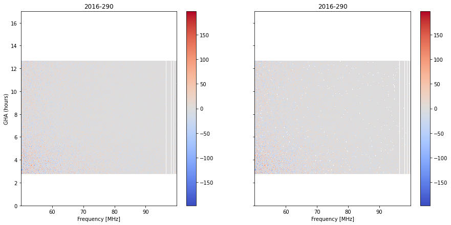
Here, we are showing the residuals as a waterfall on the left (with flags corresponding to the output of the previous step, but averaged). On the right shows the flags after flagging on the averaged data. We can see several new flags showing up.
To get a closer look at each day, and whether any days are really screwy, we can look at the daily residuals – by default, these are averaged over the full range of GHA for each day.
[65]:
fig, ax = plt.subplots(1,2, figsize=(10, 10), sharey=True)

combo_step.plot_daily_residuals(weights='old', ax=ax[0])
combo_step.plot_daily_residuals(ax=ax[1])
plt.tight_layout();
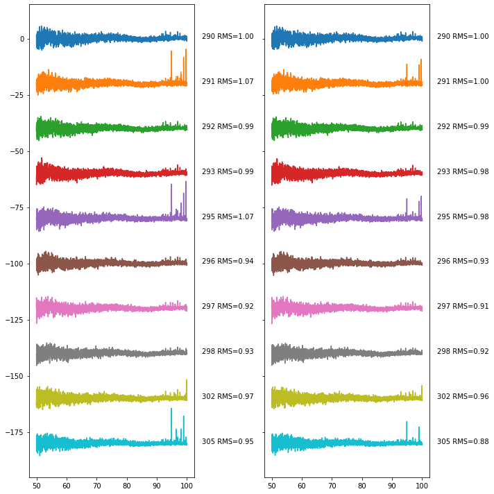
Here we again show on the left the averages performed with pre-filtered weights, while on the right it has the filtered weights. We see that the filtering at this step doesn’t seem to be particularly effective – days with poor levels of RFI to begin with still have the poorest levels of RFI after filtering. This might be an indication that we should go and run the combination step again, with different settings for the RFI.
Alternatively, this plot may indicate to us that we should look more carefully at the poorer days. We can easily show day 295 as a waterfall:
[66]:
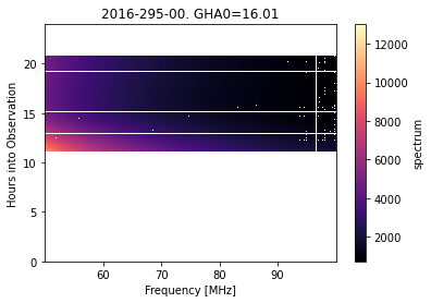
fig, ax = plt.subplots(1,2, sharey=True, figsize=(15, 7))

combo_step.plot_waterfall(day=295, quantity='resids', ax=ax[0], weights='old')
combo_step.plot_waterfall(day=295, quantity='resids', ax=ax[1], ylab=False)
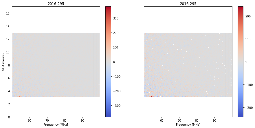
Here, looking closely, we see that there are just a few integrations where the residuals are very high, right at the bottom of the plot. Why? Let’s look at the weights:
[100]:
plt.figure(figsize=(10, 10))
combo_step.plot_waterfall(day=295, quantity='weights', flagged=False, cmap='Pastel2')
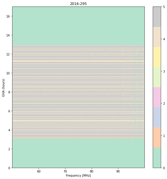
Notice that the bottom integration has on average a single sample per channel, whereas most other integrations (when they’re not completely flagged) have 4 or 5. Thus, it is just the noise level showing up.
Now, let’s say we wanted to go back from here and look at day 295 more closely before the GHA gridding. We can do this easily:
[101]:
day295 = combo_step.get_day(295)
[102]:
day295
[102]:
ModelData(filename=PosixPath('/home/smurray/edges/Steven/edges-cache/level-cache/nature-paper-subset/aux-tp-xrfi-model/linlog5-res0/2016-295-00.h5'), group_path='', require_no_extra=False)
We’ve retrieved the ModelData instance, and from there we have access to its filter step and calibration step:
[104]:
day295.filter_step.plot_waterfall();
In principle, we should dig a little further here to see if we can’t find the reason for the excess RFI, and see if we can fix it. For this tutorial, we will soldier on…
Averaging Over Days
Now we can average over all the days to really bring down the noise:
[107]:
!cat config/day_average.yml
day_range: null
ignore_days: null

xrfi_on_resids: false
xrfi_pipe:
  xrfi_model:
    model_type: linlog
    beta: -2.55
    max_iter: 15
    increase_order: true
    threshold: 4.5
    decrement_threshold: 1
    min_threshold: 3.5
    min_terms: 5
    max_terms: 7
    n_signal: 4
    n_resid: 3
    watershed: 4

  xrfi_watershed:
    tol: 0.7
The first two parameters here make it possible to ignore some of the days in the combined file (note, we can’t ignore them at the command line any more, because they’re all in one file). Then we also provide another go at RFI filtering – again, the same filtering as previously.
[108]:
!edges-analysis process day config/day_average.yml \
  -i :nature-paper-subset/aux-tp-xrfi-model/linlog5-res0/3min-bins-xrfi-model \
  -l all-days
╔══════════════════════════════════════════════════════════════════════════════╗
║                              edges-analysis day                              ║
╚══════════════════════════════════════════════════════════════════════════════╝
────────────────────────────────── Setting Up ──────────────────────────────────

                                    Settings
┏━━━━━━━━━━━━━━━━┳━━━━━━━━━━━━━━━━━━━━━━━━━━━━━━━━━━━━━━━━━━━━━━━━━━━━━━━━━━━━━┓
┃ day_range      ┃ None                                                        ┃
│ ignore_days    │ None                                                        │
│ xrfi_on_resids │ False                                                       │
│ xrfi_pipe      │ {'xrfi_model': {'model_type': 'linlog', 'beta': -2.55,      │
│                │ 'max_iter': 15, 'increase_order': True, 'threshold': 4.5,   │
│                │ 'decrement_threshold': 1, 'min_threshold': 3.5,             │
│                │ 'min_terms': 5, 'max_terms': 7, 'n_signal': 4, 'n_resid':   │
│                │ 3, 'watershed': 4}, 'xrfi_watershed': {'tol': 0.7}}         │
└────────────────┴─────────────────────────────────────────────────────────────┘

Input Files:
   /home/smurray/edges/Steven/edges-cache/level-cache/nature-paper-subset/aux-tp
-xrfi-model/linlog5-res0/3min-bins-xrfi-model/all-files.h5

Output Directory: /home/smurray/edges/Steven/edges-cache/level-cache/nature-pape
r-subset/aux-tp-xrfi-model/linlog5-res0/3min-bins-xrfi-model/all-days

───────────────────────────── Beginning Processing ─────────────────────────────
INFO     Integrating over nights...
/data4/smurray/Projects/radio/EOR/Edges/edges-analysis/src/edges_analysis/analysis/levels.py:2625: RuntimeWarning: Mean of empty slice
  params = np.nanmean(prev_step.ancillary["model_params"], axis=0)
INFO     Running xRFI...
bool
INFO     After xrfi_model, nflags=1073735/2785280 (38.6%)
bool
INFO     After xrfi_watershed, nflags=1075768/2785280 (38.6%)
INFO     ... took 14.07 sec.
─────────────────────────────── Done Processing ────────────────────────────────

Output Files:
        /home/smurray/edges/Steven/edges-cache/level-cache/nature-paper-subset/a
ux-tp-xrfi-model/linlog5-res0/3min-bins-xrfi-model/all-days/all-files.h5
Let’s read it in:
[109]:
day_step = read_step("/home/smurray/edges/Steven/edges-cache/level-cache/nature-paper-subset/aux-tp-xrfi-model/linlog5-res0/3min-bins-xrfi-model/all-days/all-files.h5")
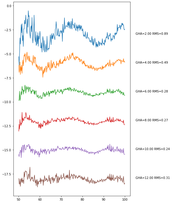
One of the useful plots you can make at this level is a per-gha-bin residual plot:
[112]:
day_step.plot_resids()
/data4/smurray/Projects/radio/EOR/Edges/edges-analysis/src/edges_analysis/analysis/tools.py:843: RuntimeWarning: Mean of empty slice
  params_out[i] = np.nanmean(these_params, axis=0)
[112]:
<AxesSubplot:>
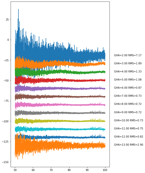
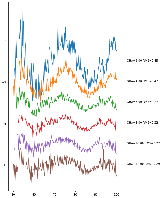
You can look at the underlying structure more closely by plotting at a lower frequency resolution:
[113]:
day_step.plot_resids(freq_resolution=0.4)
/data4/smurray/Projects/radio/EOR/Edges/edges-analysis/src/edges_analysis/analysis/tools.py:843: RuntimeWarning: Mean of empty slice
  params_out[i] = np.nanmean(these_params, axis=0)
[113]:
<AxesSubplot:>
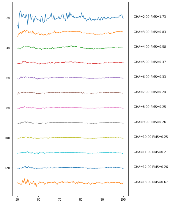
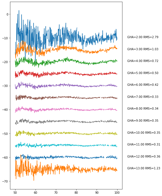
You can even change the GHA bin size:
[115]:
day_step.plot_resids(freq_resolution=0.2, gha_bin_size=2, separation=3)
/data4/smurray/Projects/radio/EOR/Edges/edges-analysis/src/edges_analysis/analysis/tools.py:843: RuntimeWarning: Mean of empty slice
  params_out[i] = np.nanmean(these_params, axis=0)
[115]:
<AxesSubplot:>
Here, one can see some likely RFI above 90 MHz. We can attempt to remove that in the final step: binning. Essentially, binning does the same thing as we just did to make this plot, but it makes a standalone object out of it (and allows for extra flagging).
Binning
We’re going to do three rounds of binning, so that we can catch extra RFI. First, we’ll bin into one-hour blocks with frequency resolution of 0.1, then we’ll move to four-hour blocks with resolution 0.4, then finally, a single spectrum.
We’ll do the first binning at the command-line:
[118]:
!cat config/binning_1.yml
freq_resolution: 0.1
gha_bin_size: 1.0

xrfi_on_resids: true
xrfi_pipe:
  xrfi_model_sweep:
    max_iter: 10
    threshold: 3.5
    which_bin: all
    watershed: 1
    window_width: 100

n_threads: 32
In this case, we use a different filter – xrfi_model_sweep, which passes a polynomial over the residuals in a sliding window, iteratively flagging in much the same way as the overall xrfi_model. This is a bit slower, but now that our data is averaged down, it should be reasonably quick.
[124]:
!edges-analysis process bin config/binning_1.yml \
  -i :nature-paper-subset/aux-tp-xrfi-model/linlog5-res0/3min-bins-xrfi-model/all-days \
  -l 1hour-100kHz
╔══════════════════════════════════════════════════════════════════════════════╗
║                              edges-analysis bin                              ║
╚══════════════════════════════════════════════════════════════════════════════╝
────────────────────────────────── Setting Up ──────────────────────────────────

                                    Settings
┏━━━━━━━━━━━━━━━━━┳━━━━━━━━━━━━━━━━━━━━━━━━━━━━━━━━━━━━━━━━━━━━━━━━━━━━━━━━━━━━┓
┃ freq_resolution ┃ 0.1                                                        ┃
│ gha_bin_size    │ 1.0                                                        │
│ xrfi_on_resids  │ True                                                       │
│ xrfi_pipe       │ {'xrfi_model_sweep': {'max_iter': 10, 'threshold': 3.5,    │
│                 │ 'which_bin': 'all', 'watershed': 1, 'window_width': 100}}  │
│ n_threads       │ 32                                                         │
└─────────────────┴────────────────────────────────────────────────────────────┘

Input Files:
   /home/smurray/edges/Steven/edges-cache/level-cache/nature-paper-subset/aux-tp
-xrfi-model/linlog5-res0/3min-bins-xrfi-model/all-days/all-files.h5

Output Directory: /home/smurray/edges/Steven/edges-cache/level-cache/nature-pape
r-subset/aux-tp-xrfi-model/linlog5-res0/3min-bins-xrfi-model/all-days/1hour-100k
Hz

───────────────────────────── Beginning Processing ─────────────────────────────
INFO     Averaging in frequency bins...
INFO     .... produced 512 frequency bins.
INFO     Averaging into 24 GHA bins.
/data4/smurray/Projects/radio/EOR/Edges/edges-analysis/src/edges_analysis/analysis/tools.py:843: RuntimeWarning: Mean of empty slice
  params_out[i] = np.nanmean(these_params, axis=0)
INFO     Running xRFI...
bool
INFO     After xrfi_model_sweep, nflags=6360/12288 (51.8%)
─────────────────────────────── Done Processing ────────────────────────────────

Output Files:
        /home/smurray/edges/Steven/edges-cache/level-cache/nature-paper-subset/a
ux-tp-xrfi-model/linlog5-res0/3min-bins-xrfi-model/all-days/1hour-100kHz/all-fil
es.h5
[134]:
bin_data = read_step("/home/smurray/edges/Steven/edges-cache/level-cache/nature-paper-subset/aux-tp-xrfi-model/linlog5-res0/3min-bins-xrfi-model/all-days/1hour-100kHz/all-files.h5")
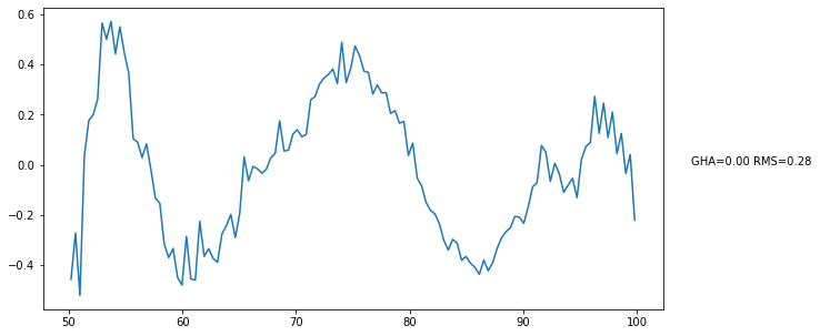
[138]:
bin_data.plot_resids(separation=5);
Things look fairly reasonable and flat. Let’s average down again, but this time, we’ll just do it dynamically:
[129]:
import yaml
with open("config/binning_1.yml") as fl:
    settings = yaml.load(fl, Loader=yaml.FullLoader)
[131]:
settings['freq_resolution'] = 0.2
settings['gha_bin_size'] = 2.0
[150]:
bin_data_2 = bin_data.promote(bin_data, **settings)
/data4/smurray/Projects/radio/EOR/Edges/edges-analysis/src/edges_analysis/analysis/tools.py:843: RuntimeWarning: Mean of empty slice
  params_out[i] = np.nanmean(these_params, axis=0)
bool
[139]:
bin_data_2.plot_resids(separation=1);
And again:
[141]:
new_settings = deepcopy(settings)
[142]:
new_settings['freq_resolution'] = 0.4
new_settings['gha_bin_size'] = 24
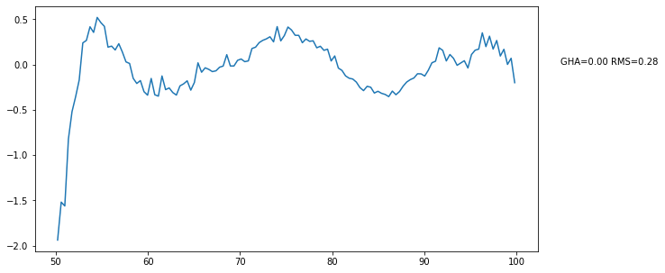
[151]:
bin_data_3 = bin_data.promote(bin_data_2, **new_settings)
bool
[152]:
plt.figure(figsize=(10, 5))
bin_data_3.plot_resids(ax=plt.gca());
These residuals are just the averaged residuals from our initial model – what happens if we refit them?
[153]:
from edges_cal.modelling import LinLog

plt.figure(figsize=(10, 5))
linlog5 = LinLog(n_terms=5, default_x=bin_data_3.raw_frequencies)

bin_data_3.plot_resids(ax=plt.gca(), refit_model=linlog5);
Round Up
We’ve now gone through the whole process. Having gone through it, you’ll notice that some steps are more useful than others for initial viewing. The calibration step is useful to look at to ensure nothing went completely bonkers with the calibration. But after that, you likely want to take it all the way through to the combination step, have a look for outliers there, and track it back into its parents using the get_day() method. After that, it’s really useful to have a look after the day
average, and try different binning schemes dynamically, looking at the residuals.
Recall also that even right from the end, we can get back to the initial steps:
[155]:
bin_data_3.combination_step
[155]:
CombinedData(filename=PosixPath('/home/smurray/edges/Steven/edges-cache/level-cache/nature-paper-subset/aux-tp-xrfi-model/linlog5-res0/3min-bins-xrfi-model/all-files.h5'), group_path='', require_no_extra=False)
[156]:
bin_data_3.get_day(295).calibration_step
[156]:
CalibratedData(filename=PosixPath('/home/smurray/edges/Steven/edges-cache/level-cache/nature-paper-subset/2016-295-00.h5'), group_path='', require_no_extra=False)