Using alanmode to reproduce the Bowman+2018 calibration

In this demo, we show how to use the alanmode sub-package, which is included in edges-analysis purely for the purpose of reroducing much of the interface of the legacy C code used to generate the results published in Bowman+2018.

Note that alanmode is not intended to be the main way of using the edges-analysis pipeline, and it is fairly restrictive in what it offers, specifically because it is trying to make it easy to match the legacy code without making mistakes. The parameter names are also not very pythonic (and sometimes not very intelligible), but are kept matching the corresponding names in the legacy interface, in order to make it easier to cross-compare.

For these reasons, this demo is essentialy an “internal” EDGES document, useful for those who have the legacy pipeline available (to be fair, the legacy pipeline is publicly available: https://github.com/edges-collab/alans-pipeline, and it contains a version of this very demo that is less instructive and more detailed.

The Data

In this demo we will be using the raw calibration data that was used to obtain the calirbation solutions for Bowman+2018 (in particular the H2 case of Figure 2). We provide convenience methods in the edges package to download these datasets. The results of this download will be cached – the first run of this tutorial will take a little while, since the spectra are almost 4 GB in size.

Throughout this demo we make plots of the various calibration quantities compared to the results of the legacy pipeline. The outputs of the legacy pipeline are publicly available, and we also provide a convenience function for obtaining them. These outputs exactly match those produced with nature-paper-case-h2. The C-code was run according to the README of the alans-pipeline repo, specifically by running the scripts/run-H2-cal C-shell script.

from edges.data import fetch_b18cal_spectra, fetch_b18cal_calibrated_s11s, fetch_b18_cal_outputs

raw_spectra_dir = fetch_b18cal_spectra()
legacy_outputs_dir = fetch_b18_cal_outputs()
raw_s11_path = fetch_b18cal_calibrated_s11s()

Using alanmode

from pathlib import Path
import numpy as np
from astropy import units as un
import matplotlib.pyplot as plt

plt.style.use("dark_background")

You can use alanmode either via a simple CLI, or as a library. Here, we will show how to use the library functions. Internally, alanmode simply combines the input parameters to manually construct a CalibrationObservation and from that determines a Calibrator instance. In general, the intention is that you would construct both of these objects yourself, with the greater flexibility afforded by working directly with the objects and their constructor methods.

# The important function:
from edges.alanmode import alancal

# Classes defining sets of parameters to pass
from edges.alanmode import EdgesScriptParams, Edges2CalobsParams, ACQPlot7aMoonParams

# Functions for reading the outputs of the legacy pipeline
from edges.alanmode import read_modelled_s11s, read_spec_txt, read_specal, LOADMAP, SPEC_LOADMAP

The alancal function is the single entry point you need to run a full receiver calibration. The function takes three main arguments, each of which is a set of parameters. The first is the defparams, which tells the function where to find the data files it needs, the second is the acqparams, which tells the function how to deal with the load spectra (which data to average, and how to downsample it), and the third is the calparams which are parameters used in the actual calibration, including the order of various S11 models, frequency range in which to find calibration solutions, and number of terms for the receiver temperature models.

Here, we specify each required parameter in full. Note that on a first run, the spectrum ACQ files need to be read, which can take a minute or so. On a second run, the averaged spectra are read in and this is very fast. However you must be careful to specify redo_spectra=True if you change any of the ACQPlot7aMoonParams or else you’ll get inconsistent results.

calobs, calibrator, s11_models, rcv_model, hot_load_loss = alancal(
    defparams = Edges2CalobsParams(
        s11_path = raw_s11_path,
        ambient_acqs = sorted(raw_spectra_dir.glob("Ambient*.acq")),
        hotload_acqs = sorted(raw_spectra_dir.glob("HotLoad*.acq")),
        open_acqs = sorted(raw_spectra_dir.glob("LongCableOpen*.acq")),
        short_acqs = sorted(raw_spectra_dir.glob("LongCableShort*.acq")),
    ),
    acqparams=ACQPlot7aMoonParams(
        delaystart=7200,
        smooth=8,
        fstart=40.0,
        fstop=110.0,
        tload=300.0,
        tcal=1000.0,
        tstart=0,
        tstop=23,
    ),
    calparams=EdgesScriptParams(
        cfit=6,
        wfit=5,
        Lh=-2,
        wfstart=50.0,
        wfstop=100.0,
        tcold=296,
        thot=399,
        nfit2=27,
        nfit3=11,
        lna_poly=0
    ),
)

Since the Bowman+2018 results are one of the main motivations for having alanmode at all, we also provide convenience methods for setting up the parameters with these parameters as defaults:

calobs_default, calibrator_default, *_ = alancal(
    defparams = Edges2CalobsParams(
        s11_path = raw_s11_path,
        ambient_acqs = sorted(raw_spectra_dir.glob("Ambient*.acq")),
        hotload_acqs = sorted(raw_spectra_dir.glob("HotLoad*.acq")),
        open_acqs = sorted(raw_spectra_dir.glob("LongCableOpen*.acq")),
        short_acqs = sorted(raw_spectra_dir.glob("LongCableShort*.acq")),
    ),
    acqparams=ACQPlot7aMoonParams.bowman_2018_defaults(),
    calparams=EdgesScriptParams.bowman_2018_defaults(),
)

We can check that these are the same:

calibrator_default == calibrator

True

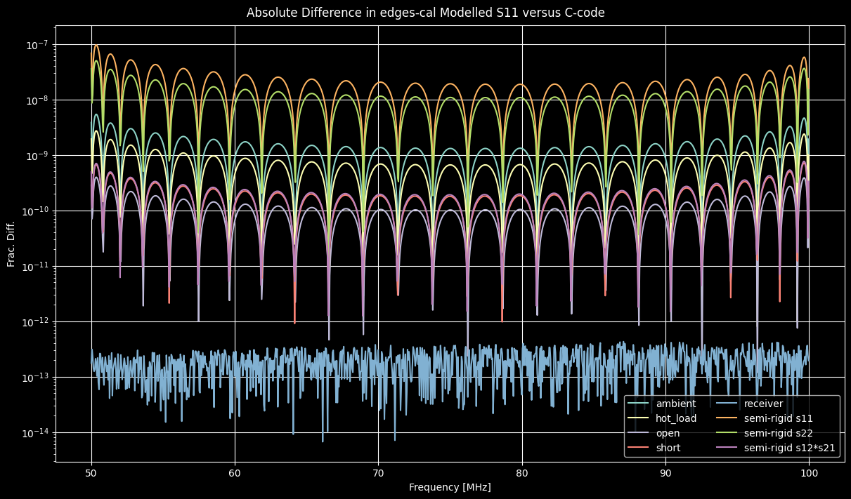
Check Modelling of S11’s

legacy_case = legacy_outputs_dir / "H2Case-fittpfix"

legacy_s11m = read_modelled_s11s(legacy_case/ "s11_modelled.txt")

The legacy pipeline outputs the modelled S11 files before cutting down the frequency range to the final calibration frequencies. While the alancal function performs the modelling and cutting in the same sequence as the legacy code, the final modelled S11’s we have access to are already cut. So here we cut the S11’s from the legacy pipeline:

mask = (legacy_s11m['freqs']>=50*un.MHz) & (legacy_s11m['freqs']<=100*un.MHz)

legacy_s11m = legacy_s11m[mask]

fig, ax = plt.subplots(1, 1, sharex=True, constrained_layout=True, figsize=(12, 7))

for i, (name, load) in enumerate(calobs.loads.items()):
    ax.plot(calobs.freqs, np.abs(load.s11.s11 - legacy_s11m[name])/np.abs(legacy_s11m[name]), label=name)

ax.set_yscale('log')
ax.set_ylabel("Frac. Diff.")

# Also plot the semi-rigid and receiver S11's
ax.plot(calobs.freqs, np.abs(calobs.receiver.s11 - legacy_s11m['receiver'])/np.abs(legacy_s11m['receiver']), label='receiver')
sp = hot_load_loss.sparams
ax.plot(calobs.freqs, np.abs(sp.s11 - legacy_s11m['semi_rigid s11'])/np.abs(legacy_s11m['semi_rigid s11']), label=f'semi-rigid s11')
ax.plot(calobs.freqs, np.abs(sp.s22 - legacy_s11m['semi_rigid s22'])/np.abs(legacy_s11m['semi_rigid s22']), label=f'semi-rigid s22')
ax.plot(calobs.freqs, np.abs(sp.s12**2 - legacy_s11m['semi_rigid s12'])/np.abs(legacy_s11m['semi_rigid s12']), label=f'semi-rigid s12*s21')


ax.legend(ncols=2)
ax.grid(True)
ax.set_xlabel("Frequency [MHz]")
fig.suptitle("Absolute Difference in edges-cal Modelled S11 versus C-code");

Check Spectrum Averaging

Now we turn to checking the averaged spectrum values. First, we define a function to read all of averaged spectrum files produced by the legacy pipeline. This simply wraps a function already provided by edges.alanmode (i.e. read_spec_txt), and puts the outputs into a nice dictionary with keys that match the conventions of edges.

Furthermore, note that, like the modelled S11s, the averaged spectra are written to file in the legacy pipeline before they are cut out to the final calibration frequency range (wfstart, wfstop). While we match the same sequence of frequency range cutting in alancal, the final spectra we have access to (without undue effort) have been cut, so we cut down the legacy values to the same range. The values outside this range are of no consequence to the calibration in any case.

def read_all_avspec(direc: Path, flow, fhigh):
    spec = {}
    allfiles = direc.glob("spe_*r.txt")
    for fl in allfiles:
        load = SPEC_LOADMAP[fl.name.split("_")[1][:-5]]
        s = read_spec_txt(fl)
        freq = s.freqs
        mask = (freq >= flow) * (freq <= fhigh)
        spec[load] = s.data.squeeze()[mask]

    return freq[mask], spec

spfreq, legacy_spec = read_all_avspec(legacy_case, flow=calobs.freqs.min(), fhigh=calobs.freqs.max())

for i, load in enumerate(legacy_spec):
    plt.plot(
        calobs.freqs,
        calobs.averaged_spectrum(calobs.loads[load], t_load=300, t_load_ns=1000) - legacy_spec[load],
        label=load
    )
plt.legend(ncols=2)
plt.ylabel("Difference [K]")
plt.xlabel("Frequency [MHz]")
plt.title("Raw spectra differences")

Text(0.5, 1.0, 'Raw spectra differences')

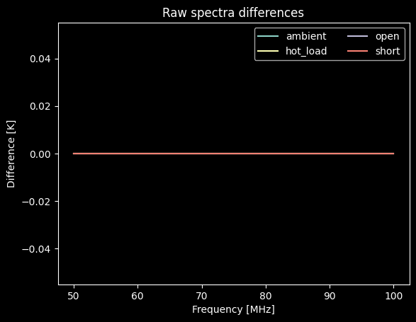
Nicely enough, all four loads have differences of exactly zero compared to the legacy code. NOTE however that this exact correspondence is achieved due to a rounding of the values to 6 decimal places upon writing the files in the legacy pipeline. Since that pipeline uses these files for further processing (instead of passing the original values in memory onto the calibration), we mimick that effect in alancal by rounding the spectrum values.

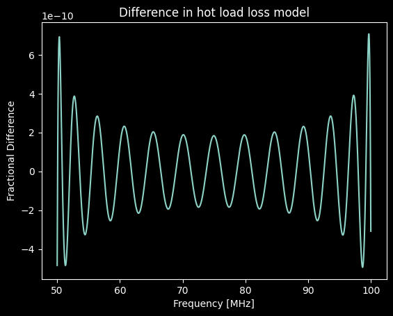
Check Hot Load Loss

legacy_loss = np.genfromtxt(legacy_case / "hot_load_loss.txt")

plt.plot(calobs.freqs, calobs.hot_load.loss / legacy_loss[mask, 1] - 1)
plt.xlabel("Frequency [MHz]")
plt.ylabel("Fractional Difference")
plt.title("Difference in hot load loss model")

Text(0.5, 1.0, 'Difference in hot load loss model')

Check Calibration Coefficients

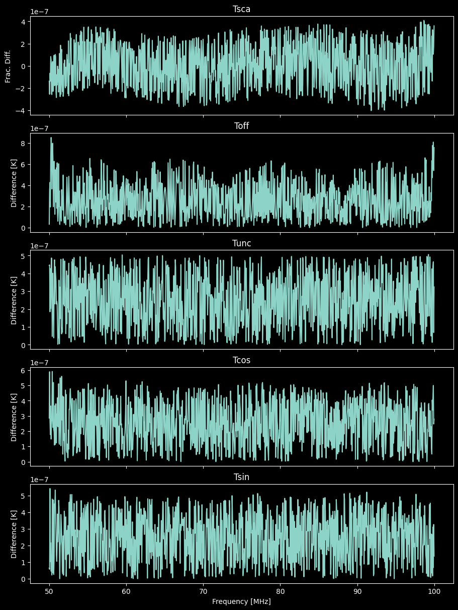
Now we finally turn to the end-products: the calibration temperatures. The output calbration solutions from the legacy pipeline specify the scale/offset temperatures in terms of their deviation from initial guesses, t_load_ns and t_load respectively. We pass the values of these guesses (defined when we ran alancal) to bring the outputs into line with the standard specification of the edges code, which are Tsca and Toff.

legacy_calibrator = read_specal(legacy_case / "specal.txt", t_load=300, t_load_ns=1000)

caltemps = ['Tsca', 'Toff', 'Tunc', 'Tcos', 'Tsin']

fig, ax = plt.subplots(len(caltemps), 1, sharex=True, constrained_layout=True, figsize=(9, 12))


for i, name in enumerate(caltemps):
    if name=='Tsca':
        # Scaling temperature, plot the ratio
        ax[i].plot(calobs.freqs, np.abs(getattr(calibrator, name) / getattr(legacy_calibrator, name)) - 1)
        ax[i].set_ylabel("Frac. Diff.")
    else:
        ax[i].plot(calobs.freqs, np.abs(getattr(calibrator, name) - getattr(legacy_calibrator, name)))
        ax[i].set_ylabel("Difference [K]")

    ax[i].set_title(name)


ax[-1].set_xlabel("Frequency [MHz]");